笔记
单击此处 下载完整的示例代码
情节的生命周期#
本教程旨在使用 Matplotlib 展示单个可视化的开始、中间和结束。我们将从一些原始数据开始,最后保存一个定制的可视化图形。在此过程中,我们尝试强调一些使用 Matplotlib 的简洁功能和最佳实践。
笔记
本教程基于 Chris Moffitt 的这篇出色的博客文章 。它由 Chris Holdgraf 转化为本教程。
关于显式与隐式接口的注释#
Matplotlib 有两个接口。有关显式和隐式接口之间权衡的解释,请参阅Matplotlib 应用程序接口 (API)。
在显式的面向对象 (OO) 界面中,我们直接利用
的实例axes.Axes在 的实例中构建可视化
figure.Figure。在受 MATLAB 启发和建模的隐式接口中,使用封装在
pyplot模块中的基于全局状态的接口来绘制到“当前轴”。请参阅pyplot 教程以更深入地了解 pyplot 界面。
大多数术语都很简单,但要记住的主要内容是:
该图是可能包含 1 个或多个 Axes 的最终图像。
轴代表一个单独的图(不要将其与“轴”一词混淆,“轴”指的是图的 x/y 轴)。
我们调用直接从 Axes 进行绘图的方法,这为我们定制绘图提供了更大的灵活性和能力。
笔记
一般来说,显式接口优于隐式 pyplot 接口进行绘图。
我们的数据#
我们将使用源自本教程的帖子中的数据。它包含许多公司的销售信息。
import numpy as np
import matplotlib.pyplot as plt


data = {'Barton LLC': 109438.50,
        'Frami, Hills and Schmidt': 103569.59,
        'Fritsch, Russel and Anderson': 112214.71,
        'Jerde-Hilpert': 112591.43,
        'Keeling LLC': 100934.30,
        'Koepp Ltd': 103660.54,
        'Kulas Inc': 137351.96,
        'Trantow-Barrows': 123381.38,
        'White-Trantow': 135841.99,
        'Will LLC': 104437.60}
group_data = list(data.values())
group_names = list(data.keys())
group_mean = np.mean(group_data)
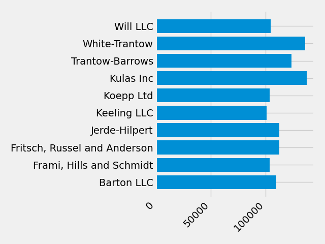
开始#
该数据自然地可视化为条形图,每组一个条形图。要使用面向对象的方法做到这一点,我们首先生成一个figure.Figure和
的实例axes.Axes。图就像画布,轴是画布的一部分,我们将在其上进行特定的可视化。
笔记
图形上可以有多个轴。有关如何执行此操作的信息,请参阅紧密布局教程。
fig, ax = plt.subplots()
现在我们有了一个 Axes 实例,我们可以在它上面绘图。
fig, ax = plt.subplots()
ax.barh(group_names, group_data)
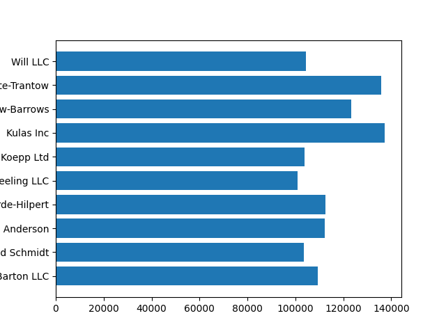
<BarContainer object of 10 artists>
控制风格#
Matplotlib 中有许多样式可供您根据需要定制可视化。要查看样式列表,我们可以使用
style.
print(plt.style.available)
['Solarize_Light2', '_classic_test_patch', '_mpl-gallery', '_mpl-gallery-nogrid', 'bmh', 'classic', 'dark_background', 'fast', 'fivethirtyeight', 'ggplot', 'grayscale', 'seaborn-v0_8', 'seaborn-v0_8-bright', 'seaborn-v0_8-colorblind', 'seaborn-v0_8-dark', 'seaborn-v0_8-dark-palette', 'seaborn-v0_8-darkgrid', 'seaborn-v0_8-deep', 'seaborn-v0_8-muted', 'seaborn-v0_8-notebook', 'seaborn-v0_8-paper', 'seaborn-v0_8-pastel', 'seaborn-v0_8-poster', 'seaborn-v0_8-talk', 'seaborn-v0_8-ticks', 'seaborn-v0_8-white', 'seaborn-v0_8-whitegrid', 'tableau-colorblind10']
您可以使用以下方式激活样式:
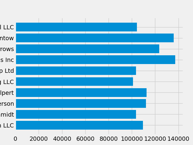
plt.style.use('fivethirtyeight')
现在让我们重新制作上面的图,看看它的样子:
fig, ax = plt.subplots()
ax.barh(group_names, group_data)

<BarContainer object of 10 artists>
样式控制很多东西,例如颜色、线宽、背景等。
自定义绘图#
现在我们已经有了一个我们想要的具有一般外观的图,所以让我们对其进行微调,以便它可以打印。首先让我们旋转 x 轴上的标签,使它们显示得更清楚。我们可以通过以下方法访问这些标签axes.Axes.get_xticklabels():
fig, ax = plt.subplots()
ax.barh(group_names, group_data)
labels = ax.get_xticklabels()
如果我们想一次设置多个项目的属性,使用该pyplot.setp()函数很有用。这将采用 Matplotlib 对象的列表(或多个列表),并尝试为每个对象设置一些样式元素。
fig, ax = plt.subplots()
ax.barh(group_names, group_data)
labels = ax.get_xticklabels()
plt.setp(labels, rotation=45, horizontalalignment='right')
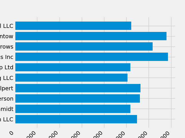
[None, None, None, None, None, None, None, None, None, None, None, None, None, None, None, None, None, None, None, None, None, None, None, None, None, None, None]
看起来这切断了底部的一些标签。我们可以告诉 Matplotlib 自动为我们创建的图形中的元素腾出空间。为此,我们设置autolayoutrcParams 的值。有关使用 rcParams 控制绘图的样式、布局和其他功能的更多信息,请参阅
使用样式表和 rcParams 自定义 Matplotlib。
plt.rcParams.update({'figure.autolayout': True})

fig, ax = plt.subplots()
ax.barh(group_names, group_data)
labels = ax.get_xticklabels()
plt.setp(labels, rotation=45, horizontalalignment='right')
[None, None, None, None, None, None, None, None, None, None, None, None, None, None, None, None, None, None, None, None, None, None, None, None, None, None, None]
接下来,我们为绘图添加标签。要使用 OO 接口执行此操作,我们可以使用该Artist.set()方法设置此 Axes 对象的属性。
fig, ax = plt.subplots()
ax.barh(group_names, group_data)
labels = ax.get_xticklabels()
plt.setp(labels, rotation=45, horizontalalignment='right')
ax.set(xlim=[-10000, 140000], xlabel='Total Revenue', ylabel='Company',
       title='Company Revenue')
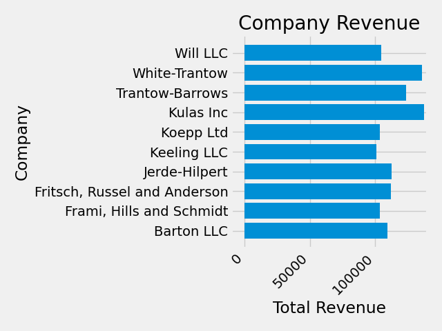
[(-10000.0, 140000.0), Text(0.5, 87.00000000000003, 'Total Revenue'), Text(86.99999999999997, 0.5, 'Company'), Text(0.5, 1.0, 'Company Revenue')]
pyplot.subplots()
我们还可以使用该函数调整此图的大小。我们可以使用figsize关键字参数来做到这一点。
笔记
NumPy 中的索引遵循形式(行、列),而figsize 关键字参数遵循形式(宽度、高度)。这遵循可视化中的约定,不幸的是与线性代数不同。
fig, ax = plt.subplots(figsize=(8, 4))
ax.barh(group_names, group_data)
labels = ax.get_xticklabels()
plt.setp(labels, rotation=45, horizontalalignment='right')
ax.set(xlim=[-10000, 140000], xlabel='Total Revenue', ylabel='Company',
       title='Company Revenue')
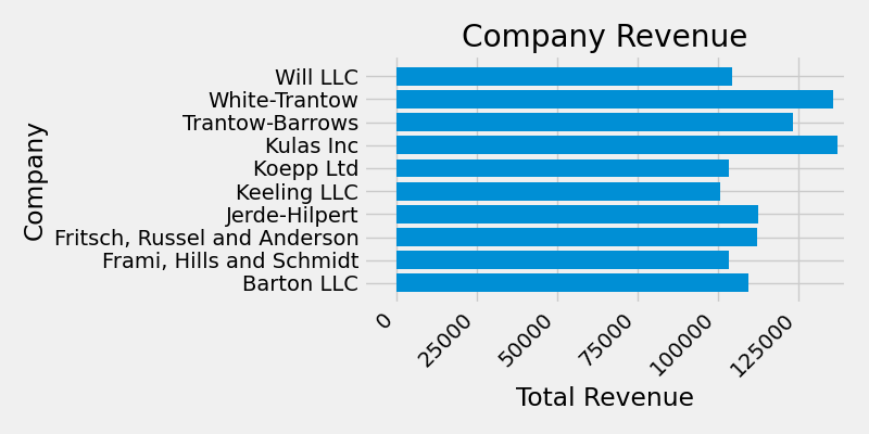
[(-10000.0, 140000.0), Text(0.5, 86.99999999999997, 'Total Revenue'), Text(86.99999999999997, 0.5, 'Company'), Text(0.5, 1.0, 'Company Revenue')]
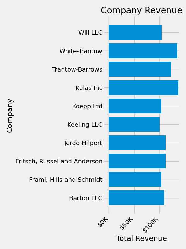
对于标签,我们可以以函数的形式指定自定义格式指南。下面我们定义一个函数,它接受一个整数作为输入,并返回一个字符串作为输出。当与Axis.set_major_formatteror
一起使用时Axis.set_minor_formatter,它们将自动创建和使用一个
ticker.FuncFormatter类。
对于此函数,x参数是原始刻度标签并且pos
是刻度位置。我们只会x在这里使用,但两个参数都是必需的。
def currency(x, pos):
    """The two arguments are the value and tick position"""
    if x >= 1e6:
        s = '${:1.1f}M'.format(x*1e-6)
    else:
        s = '${:1.0f}K'.format(x*1e-3)
    return s
然后我们可以将此函数应用于绘图上的标签。为此,我们使用xaxis轴的属性。这使您可以在我们的绘图上的特定轴上执行操作。
fig, ax = plt.subplots(figsize=(6, 8))
ax.barh(group_names, group_data)
labels = ax.get_xticklabels()
plt.setp(labels, rotation=45, horizontalalignment='right')

ax.set(xlim=[-10000, 140000], xlabel='Total Revenue', ylabel='Company',
       title='Company Revenue')
ax.xaxis.set_major_formatter(currency)
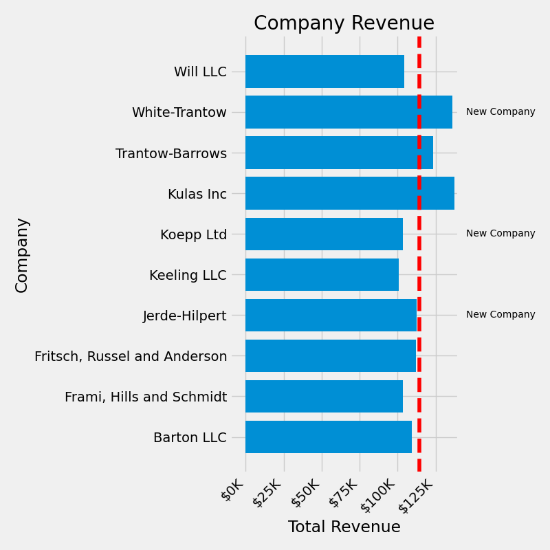
结合多个可视化#
可以在同一实例上绘制多个绘图元素
axes.Axes。为此,我们只需要在该轴对象上调用另一个绘图方法。
fig, ax = plt.subplots(figsize=(8, 8))
ax.barh(group_names, group_data)
labels = ax.get_xticklabels()
plt.setp(labels, rotation=45, horizontalalignment='right')

# Add a vertical line, here we set the style in the function call
ax.axvline(group_mean, ls='--', color='r')

# Annotate new companies
for group in [3, 5, 8]:
    ax.text(145000, group, "New Company", fontsize=10,
            verticalalignment="center")

# Now we move our title up since it's getting a little cramped
ax.title.set(y=1.05)

ax.set(xlim=[-10000, 140000], xlabel='Total Revenue', ylabel='Company',
       title='Company Revenue')
ax.xaxis.set_major_formatter(currency)
ax.set_xticks([0, 25e3, 50e3, 75e3, 100e3, 125e3])
fig.subplots_adjust(right=.1)

plt.show()
保存我们的情节#
现在我们对绘图的结果感到满意,我们想将其保存到磁盘。我们可以在 Matplotlib 中保存许多文件格式。要查看可用选项列表,请使用:
print(fig.canvas.get_supported_filetypes())
{'eps': 'Encapsulated Postscript', 'jpg': 'Joint Photographic Experts Group', 'jpeg': 'Joint Photographic Experts Group', 'pdf': 'Portable Document Format', 'pgf': 'PGF code for LaTeX', 'png': 'Portable Network Graphics', 'ps': 'Postscript', 'raw': 'Raw RGBA bitmap', 'rgba': 'Raw RGBA bitmap', 'svg': 'Scalable Vector Graphics', 'svgz': 'Scalable Vector Graphics', 'tif': 'Tagged Image File Format', 'tiff': 'Tagged Image File Format', 'webp': 'WebP Image Format'}
然后我们可以使用figure.Figure.savefig()来将图形保存到磁盘。请注意,我们在下面显示了几个有用的标志:
transparent=True如果格式支持,则使保存的图形的背景透明。dpi=80控制输出的分辨率(每平方英寸的点数)。bbox_inches="tight"使图形的边界适合我们的情节。
# Uncomment this line to save the figure.
# fig.savefig('sales.png', transparent=False, dpi=80, bbox_inches="tight")
脚本总运行时间:(0分3.918秒)